As part of my course project last semester, I had to investigate the use and functioning of Microreactors in Diagnostic applications. One of these uses is in a PCR unit, whose function is to multiply the DNA-sample in the drawn blood n-fold in order to successfully detect diseases (those which directly affect DNA of the local region).
How this is a analogous to a Chemical Engineering problem:
Scaling up v/s Numbering up
Typically, when we encounter a problem of increasing an extensive property in our system, the approach is to simply scale up the process until a target value of that property is achieved.
However, if that extensive property is the concentration of a species, an excessive amount of raw material would be required, which, more often than not is not possible in case of biological applications. However, many biological species show interesting properties, such as, the property of replication in DNA, which makes processes which include biological species worth exploring.
Flow in the Microreactor
The flow in microreactor is governed by viscous forces rather than inertial forces, this property along with the manifold increase in the surface to volume ratio in a microreactor compared to a large-scale industrial reactor motivates us to utilize microreactors where we need a high qualitative throughput with the smallest amount of raw material available. So the PCR unit is essentially like a Plug flow reactor.
Model
Overview:
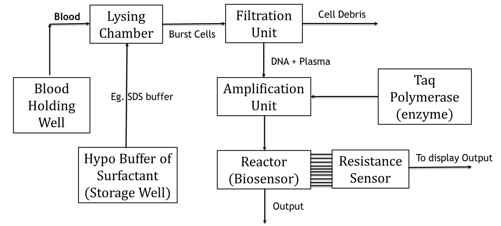
Here, we take a look at the process of detection of diseases such as Malaria, Tuberculosis etc. which is done typically via. Blood testing. And our particular model, will focus on one of these units: Amplification unit (A type of plug flow reactor) of the system
Mathematical Model of PCR
Every genome (disease injected/ human DNA) has a particular fluorescence value which, when detected, confirms the presence of a disease in the system as well as the stage of the disease depending upon the genome count. However, for all practical testing purposes, we can only draw up to a millilitre of patient’s blood, which is not enough for detection.
A DNA amplification sequence will move ahead in 3 steps as per out model:
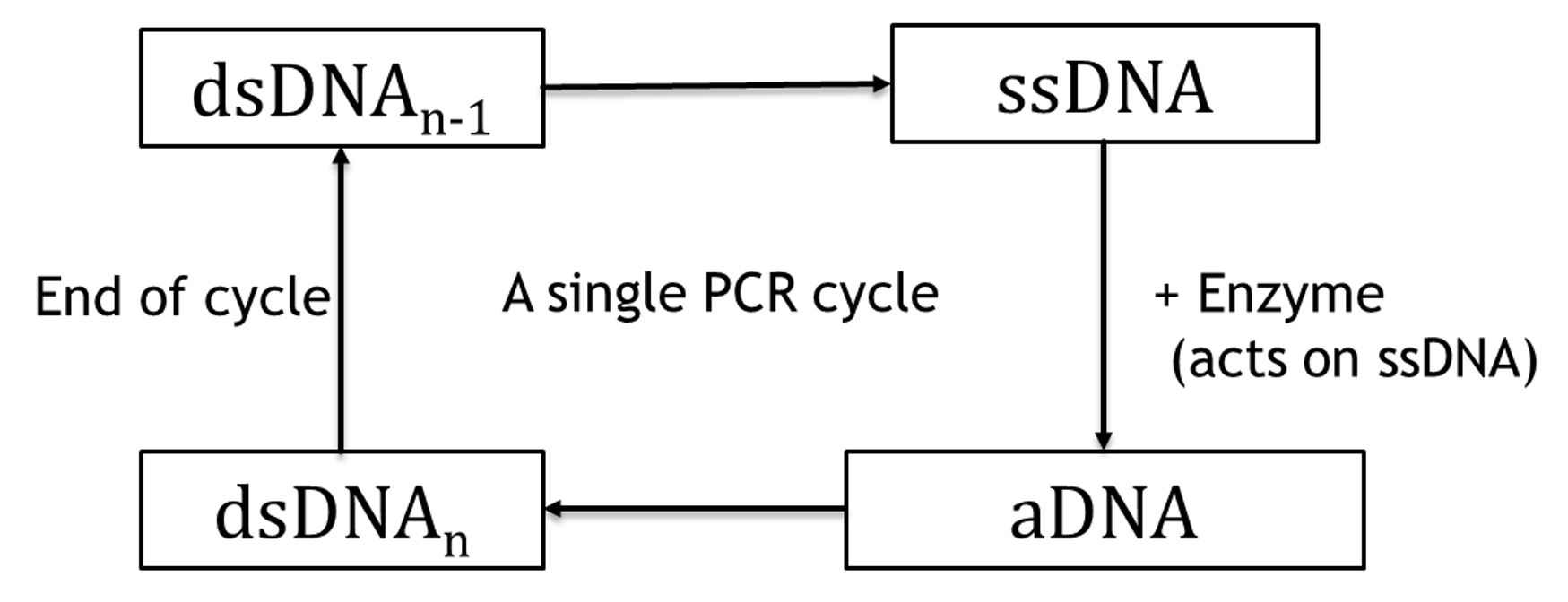
Step 1: Denaturation of Double strand DNA (dsDNA):,
dsDNA -> 2 * ssDNA (T= 368.15 K)
Step 2: Annealing of Single strand DNA (ssDNA):
ssDNA + enzyme -> aDNA (T= 328.15 K)
Step 3: Extension of Annealed DNA (aDNA):
aDNA -> dsDNA (T= 345.15 K)
All these steps have an associated efficiency(yield in this case):
Ꜫdenaturation, Ꜫannealing & Ꜫextension
Hence, we can write, after ‘n’ such PCR cycles:
[DNA]n = [DNA]0(1+Ꜫ)n
where, Ꜫ = Ꜫdenaturation * Ꜫannealing * Ꜫextension = efficiency of PCR unit
And the detected fluorescence is: Fn = α * [DNA]n Where α is the const. of proportionality dependent on the instrument used to measure the fluorescence.
Process variables: Concentration, time, efficiency Defined/ Control variables: T, ΔP
Computational Model
Using COMSOL, we have modelled the above sequence of events in a microreactor.
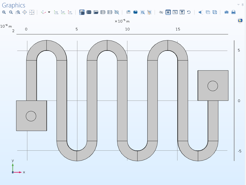
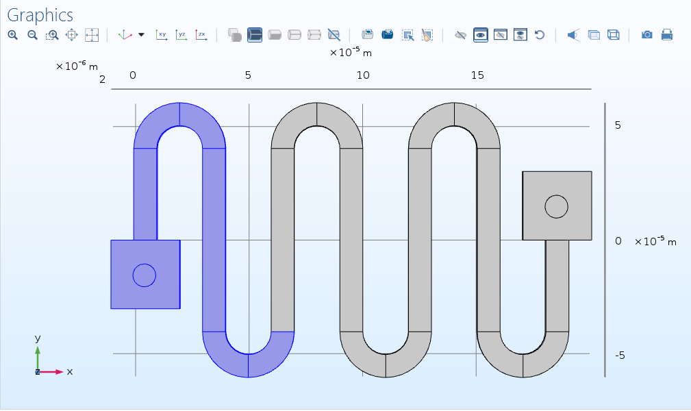
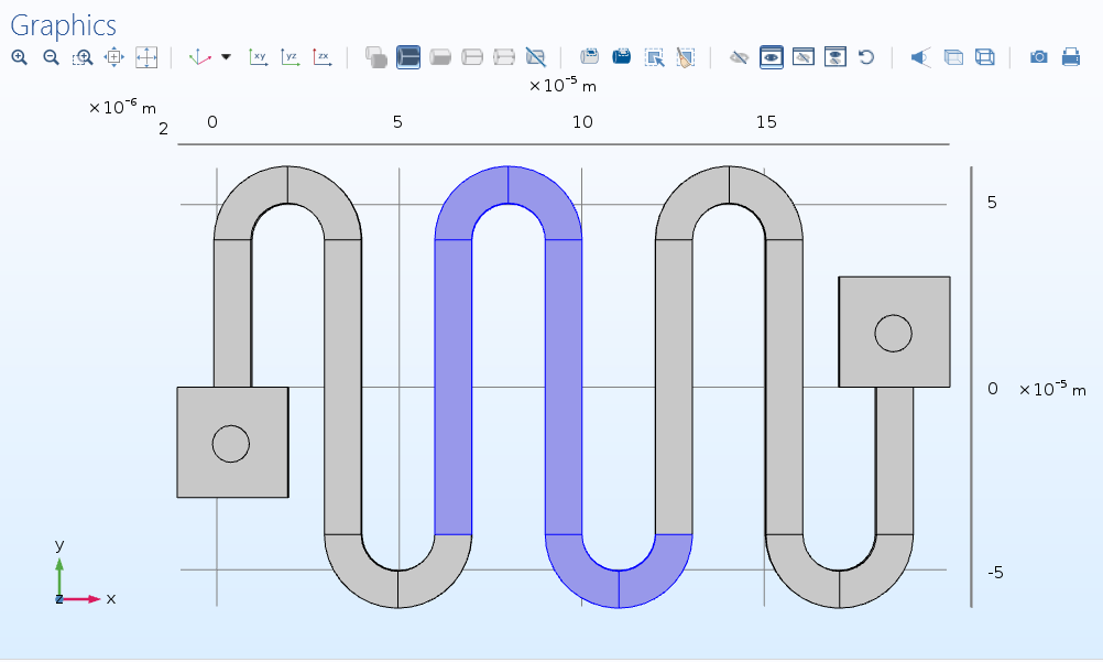
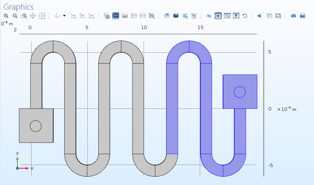
Geometry:
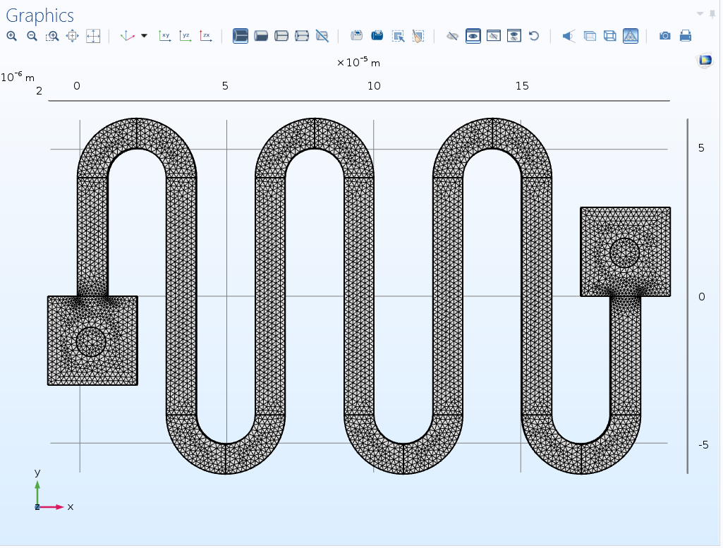
Meshing:
Physics:
Modules Used in the Software are:
-
Transport of diluted species module
-
Conjugate heat transfer Module
-
Laminar flow module
-
Non-isothermal flow Multiphysics module
To model 1 PCR cycle, we’ve divided the module in 3 different temperature zones as the 3 steps are characteristic to a temperature value.
Denaturation Zone (T= 368.15 K)
Annealing Zone (T= 328.15 K)
Extension Zone (T = 345.15 K)
Results
We ran the coupled (heat, mass and momentum) flow simulations in 2 study steps:
-
Stationary Plug flow (Temp. and velocity)
-
Time-dependent reactive flow (mass transfer)
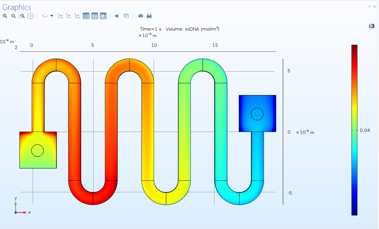
After confining reactions to temperature zones specified above, we get the following results in terms of concentration profiles through the reactor volume.
(Due to resource restriction, we limited the time for reaction to 1 second and have modelled a single PCR cycle. Also, a coarser but refined mesh was used to model Non-isothermal flow.)
Concentration of ssDNA
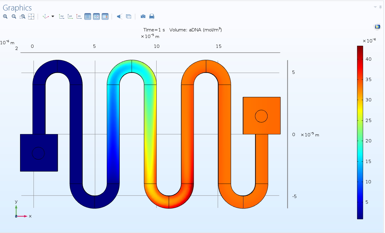
Concentration of aDNA
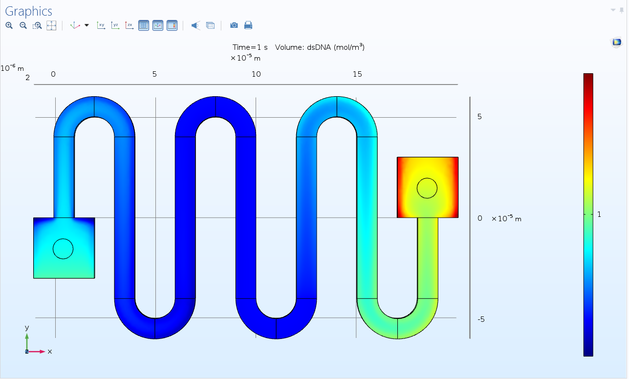
Concentration of dsDNA
• Expectedly, the value of single strand DNA increases in Zone 1 and then slowly decreases as annealing and extension takes place.
• The value of aDNA is negligible in Zone 1 and 2, increases to a value which remains constant throughout Zone 3.
The value of dsDNA, although initially low due to low concentration becomes lower in zone 1 via. Denaturation (opposite to ssDNA) but increases to a higher value after extension in Zone 3, indicating multiplication of dsDNA w.r.t. initial value. ( A higher wavelength colour indicates higher concentration value)
Hence, for 1 PCR cycle, as shown by the simulation results, Ꜫdenaturation, Ꜫannealing & Ꜫextension are all quite low but do indicate the process being taking place in the specified manner.
Conclusion & Way Ahead:
The importance of numbering up instead of scaling up: Here, we can easily see via. The small difference in order of ssDNA and dsDNA and a higher difference in order of aDNA that the efficiency of a single PCR cycle is quite low and hence in a complete PCR, this same unit is repeated to nearly 100 times in order to minimize the concentration of ssDNA and aDNA w.r.t. dsDNA.
This unit, with larger computational resources could easily be repeated for a larger spacetime domain in order to fully simulate a PCR microreactor.